ANNchor User Guide (v1.1.0)
Using ANNchor to find k-NN graphs is relatively straightforward. Let’s take a look at the general structure
import annchor

X =          #your data, list/np.array of items

distance =   #your distance function, distance(x[i],x[j]) = d

#Initialise the Annchor object with some parameters
ann = annchor.Annchor(X,
                      distance,
                      n_anchors=15,
                      n_neighbors=15)

ann.fit() #Find the k-NN graph

ann.neighbour_graph
That’s all there is to it!
Feel free to take a look at some of the examples below. Bear in mind that the run-times quoted below will vary by machine: we used a MacBook Pro with 2 GHz Quad-Core Intel i5 processor and 16 GB RAM. Any computations involving numba may want to be run twice to eliminate numba-jit compile times.
Example: Wasserstein
Wasserstein distance, also known as Earth Mover’s distance, is a metric for comparing probability distributions. Practically speaking, it is also quite useful for comparing 2D images. Unfortunately, Wasserstein can be quite slow to compute. However, this makes it perfect to demonstrate the effectiveness of ANNchor!
Let’s find the 25-NN graph for the sklearn digits dataset (from the UCI ML repository), under the Wasserstein metric. We’ll compare three methods: brute force, nearest neighbour descent, and ANNchor.
Let’s start by importing some useful packages.
import numpy as np
import time
import matplotlib.pyplot as plt

from annchor import Annchor, BruteForce, compare_neighbor_graphs
from annchor.datasets import load_digits, load_digits_large
We’ll load the digits dataset and take a look.
k=25

data = load_digits()
X = data['X']
y = data['y']
neighbor_graph = data['neighbor_graph']
M = data['cost_matrix']

nx = X.shape[0]
print('Data set contains %d digits' % nx)

fig,axs = plt.subplots(2,5)
axs = axs.flatten()
for i,ax in enumerate(axs):
    ax.imshow(X[y==i][0].reshape(8,8))
    ax.axis('off')

plt.tight_layout(h_pad=0.1, w_pad=0.3)
plt.show()
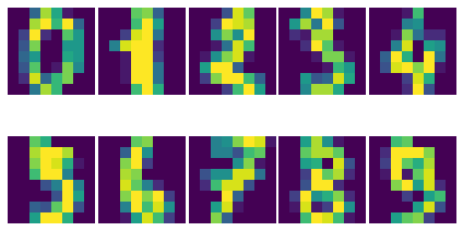
So we have a bunch of 8x8 images, 1797 to be exact. Let’s now import the Wasserstein distance. This implementation is borrowed from PyNNDescent, packaged with annchor for convenience. The cost matrix for the 8x8 images is supplied as a keyword argument.
The Wasserstein metric is quite slow to compute - compare it to the Euclidean metric on our data.
from pynndescent.distances import kantorovich
# kantorovich is just another name for the wasserstein distance

randX = lambda : X[np.random.randint(nx)]
%timeit kantorovich(randX(),randX(),cost=M)
%timeit np.linalg.norm(randX()-randX())
203 µs ± 5.37 µs per loop (mean ± std. dev. of 7 runs, 1000 loops each)
12.3 µs ± 107 ns per loop (mean ± std. dev. of 7 runs, 100000 loops each)
So Wasserstein is clocking in at around 20 times slower than Euclidean: We’re firmly in the territory of slow metrics.
Brute Force Approach
If we wanted to brute-force the k-NN graph, then we must make around 1.6 million calls to the metric. Let’s try that, with a little help from numba, and see how it goes
start_time = time.time()

bruteforce = BruteForce(X,
                        'wasserstein',
                         func_kwargs = {'cost_matrix': M}
                       )
bruteforce.fit()

print('Brute Force Time: %5.3f seconds' % (time.time()-start_time))

error = compare_neighbor_graphs(neighbor_graph,
                                bruteforce.neighbor_graph,
                                k)

print('Brute Force Accuracy: %d incorrect NN pairs (%5.3f%%)' % (error,100*error/(k*nx)))
Brute Force Time: 108.233 seconds
Brute Force Accuracy: 0 incorrect NN pairs (0.000%)
Reasonably slow, but does have the merit of giving the exact answer.
Nearest Neighbor Descent
Now let’s try a state-of-the-art k-NN graph construction method, Nearest Neighbour Descent. In particular, we’ll use the PyNNDescent python implementation (which is also used in the popular python library UMAP). We should expect this to do better than the brute force method.
from pynndescent import NNDescent
from numba import njit

@njit()
def wasserstein(x, y):
    return kantorovich(x, y, cost=M)

start_time = time.time()

# Call nearest neighbour descent
nndescent = NNDescent(X,n_neighbors=k,metric=wasserstein,random_state=1)
print('PyNND Time: %5.3f seconds' % (time.time()-start_time))

# Test accuracy
error = compare_neighbor_graphs(neighbor_graph,
                                nndescent.neighbor_graph,
                                k)
print('PyNND Accuracy: %d incorrect NN pairs (%5.3f%%)' % (error,100*error/(k*nx)))
PyNND Time: 70.988 seconds
PyNND Accuracy: 23 incorrect NN pairs (0.051%)
Not bad, we trimmed 38 seconds from the run-time for a minimal hit to accuracy.
ANNchor
How does ANNchor compare? Remember, we are competing with 83s and 69s for brute force and PyNNDescent respectively. Can we do better?
start_time = time.time()

# Call ANNchor
ann = Annchor(X,
              'wasserstein',
              func_kwargs = {'cost_matrix': M},
              n_anchors=25,
              n_neighbors=k,
              n_samples=5000,
              p_work=0.16)

ann.fit()
print('ANNchor Time: %5.3f seconds' % (time.time()-start_time))

# Test accuracy
error = compare_neighbor_graphs(neighbor_graph,
                                ann.neighbor_graph,
                                k)
print('ANNchor Accuracy: %d incorrect NN pairs (%5.3f%%)' % (error,100*error/(k*nx)))
ANNchor Time: 21.311 seconds
ANNchor Accuracy: 8 incorrect NN pairs (0.018%)
Much better! We’ve got the 25-NN graph in less than half the time it took for PyNNDescent, with comparable accuracy!
A Larger Data Set
What if we up the size of the data set? The previous set was quite small, so it’s important to see what happens when things get a bit bigger. Not much bigger, of course, since we don’t want to be waiting forever to run these tests!
Let’s try the full UCI digits data set, 5620 8x8 images (https://archive.ics.uci.edu/ml/datasets/optical+recognition+of+handwritten+digits).
# Load the data
from annchor.datasets import load_digits_large

k=25

X = load_digits_large()['X']
y = load_digits_large()['y']
neighbor_graph = load_digits_large()['neighbor_graph']

nx = X.shape[0]


start_time = time.time()

# Call nearest neighbour descent
nndescent = NNDescent(X,n_neighbors=k,metric=wasserstein,random_state=1)
print('PyNND Time: %5.3f seconds' % (time.time()-start_time))

# Test accuracy
error = compare_neighbor_graphs(neighbor_graph,
                                nndescent.neighbor_graph,
                                k)
print('PyNND Accuracy: %d incorrect NN pairs (%5.3f%%)' % (error,100*error/(k*nx)))


start_time = time.time()

# Call ANNchor
ann = Annchor(X,
              wasserstein,
              n_anchors=30,
              n_neighbors=k,
              n_samples=5000,
              p_work=0.1)

ann.fit()
print('ANNchor Time: %5.3f seconds' % (time.time()-start_time))


# Test accuracy
error = compare_neighbor_graphs(neighbor_graph,
                                ann.neighbor_graph,
                                k)
print('ANNchor Accuracy: %d incorrect NN pairs (%5.3f%%)' % (error,100*error/(k*nx)))
PyNND Time: 225.864 seconds
PyNND Accuracy: 86 incorrect NN pairs (0.061%)
ANNchor Time: 105.233 seconds
ANNchor Accuracy: 77 incorrect NN pairs (0.055%)
Again, we see that ANNchor can be much quicker than state-of-the-art!
Example: Levenshtein
Levenshtein distance (or Edit distance) is a metric on strings. It is the number of insertions, substitutions and deletions required to change one word into an- other; for example, ‘cat’ is changed to ‘hat’ by substitution of the ‘c’ for an ‘h’, and thus they are Levenshtein distance one from each other. Levenshtein distance has found practical uses in a variety of fields, including natural language processing (e.g spell-check) and bioinformatics (e.g. DNA sequence similarity). While the Levenshtein distance is an intuitive metric on strings, it does come at a computational cost, especially on long strings where it can be difficult to find the minimal number of edits. This makes it another great candidate for ANNchor.
To test how well ANNchor and other k-NN algorithms perform with respect to Levenshtein distance, we constructed a string data set for benchmarking purposes. The data set consists of 1600 strings of length 400-600, with 26 possible characters (i.e. the English alphabet). The 1600 strings can be separated into 8 clusters of two distinct varieties: filaments and clouds. The clouds are generated by taking a base string (the cloud ‘centre’) and performing a number of random edits to form a new string; thus every point in a cloud is ‘close’ to the base string. The filaments are generated in a similar way: take a base string to start the filament; create a new string by making a small number of random edits to the base string, and add the new string to the filament; continue to extend the filament by adding new strings a small number of edits from the last added string. In this way, the filament is made by traversing what is essentially a 1D path through the space of strings. The clouds and filaments can be clearly seen in a UMAP projection of the string data set, shown in below.

A typical Levenshtein distance in this data set took about 33 times as long as calculating Euclidean distance on vectors of comparable length. It’s also worth noting that there aren’t any numba compiled Levenshtein routines (as of writing), which means that we can’t use PyNNDescent, or stick this problem directly into UMAP.
First we’ll import some modules and look at the data.
import os
import numpy as np
import time
from annchor.datasets import load_strings

strings_data = load_strings()
X = strings_data['X']
y = strings_data['y']
neighbor_graph = strings_data['neighbor_graph']

nx = X.shape[0]

for x in X[::100]:
    print(x[:50]+'...')
cuiojvfnseoksugfcbwzrcoxtjxrvojrguqttjpeauenefmkmv...
uiofnsosungdgrxiiprvojrgujfdttjioqunknefamhlkyihvx...
cxumzfltweskptzwnlgojkdxidrebonxcmxvbgxayoachwfcsy...
cmjpuuozflodwqvkascdyeosakdupdoeovnbgxpajotahpwaqc...
vzdiefjmblnumdjeetvbvhwgyasygrzhuckvpclnmtviobpzvy...
nziejmbmknuxdhjbgeyvwgasygrhcpdxcgnmtviubjvyzjemll...
yhdpczcjxirmebhfdueskkjjtbclvncxjrstxhqvtoyamaiyyb...
yfhwczcxakdtenvbfctugnkkkjbcvxcxjwfrgcstahaxyiooeb...
yoftbrcmmpngdfzrbyltahrfbtyowpdjrnqlnxncutdovbgabo...
tyoqbywjhdwzoufzrqyltahrefbdzyunpdypdynrmchutdvsbl...
dopgwqjiehqqhmprvhqmnlbpuwszjkjjbshqofaqeoejtcegjt...
rahobdixljmjfysmegdwyzyezulajkzloaxqnipgxhhbyoztzn...
dfgxsltkbpxvgqptghjnkaoofbwqqdnqlbbzjsqubtfwovkbsk...
pjwamicvegedmfetridbijgafupsgieffcwnmgmptjwnmwegvn...
ovitcihpokhyldkuvgahnqnmixsakzbmsipqympnxtucivgqyi...
xvepnposhktvmutozuhkbqarqsbxjrhxuumofmtyaaeesbeuhf...
Let’s look at some different ways of computing the 15-NN graph.
Brute Force
The brute force method is the same as above - compute the all-pairs distance matrix. Since we don’t have the help of numba this time round, we will use joblib to do some parallelisation.
from annchor import BruteForce
from annchor import compare_neighbor_graphs

k = 15

start_time = time.time()

bruteforce = BruteForce(X,'levenshtein')
bruteforce.get_neighbor_graph()

print('Brute Force Time: %5.3f seconds' % (time.time()-start_time))

error = compare_neighbor_graphs(neighbor_graph,
                                bruteforce.neighbor_graph,
                                k)

print('Brute Force Accuracy: %d incorrect NN pairs (%5.3f%%)' % (error,100*error/(k*nx)))
Brute Force Time: 173.302 seconds
Brute Force Accuracy: 0 incorrect NN pairs (0.000%)
Quite slow, especially when we consider that there are only 1600 strings in the data set!
HNSW (nmslib)
The nmslib implementation of HNSW is another state-of-the-art k-NN library, one of the few out there that can deal with Levenshtein distances. You might give this a go if you don’t want to do brute force, but how does it get on?
import nmslib

start_time = time.time()

CPU_COUNT = os.cpu_count()
# specify some parameters
index_time_params = {'M': 20,
                     'indexThreadQty': CPU_COUNT,
                     'efConstruction': 100,
                     'post' : 2}

# create the index
index = nmslib.init(method='hnsw',
                    space='leven',
                    dtype=nmslib.DistType.INT,
                    data_type=nmslib.DataType.OBJECT_AS_STRING)

index.addDataPointBatch(data=list(X))
index.createIndex(index_time_params,print_progress=True)

# query the index
res = index.knnQueryBatch(list(X), k=k, num_threads=CPU_COUNT)
hnsw_neighbor_graph = [np.array([x[0]for x in res]),np.array([x[1]for x in res])]
print('HNSW Time: %5.3f seconds' % (time.time()-start_time))


error = compare_neighbor_graphs(neighbor_graph,
                                hnsw_neighbor_graph,
                                k)

print('HNSW Accuracy: %d incorrect NN pairs (%5.3f%%)' % (error,100*error/(k*nx)))
HNSW Time: 288.078 seconds
HNSW Accuracy: 9 incorrect NN pairs (0.037%)
Slower than brute force! What’s going on here? Well, it turns out that nmslib’s HNSW Levenshtein implementation only really shines when the data set is large and the strings are short. It also boasts quick query times once the index has been created; but for k-NN graph construction the index creation time is very important.
ANNchor
Now it’s ANNchor’s turn! How does it do?
start_time = time.time()
ann = Annchor(X,
              'levenshtein',
              n_anchors=23,
              n_neighbors=k,
              random_seed=5,
              n_samples=5000,
              p_work=0.12,
              niters=4)

ann.fit()
print('ANNchor Time: %5.3f seconds' % (time.time()-start_time))


# Test accuracy
error = compare_neighbor_graphs(neighbor_graph,
                                ann.neighbor_graph,
                                k)
print('ANNchor Accuracy: %d incorrect NN pairs (%5.3f%%)' % (error,100*error/(k*nx)))
ANNchor Time: 28.269 seconds
ANNchor Accuracy: 0 incorrect NN pairs (0.000%)
Super speedy, and accurate too!
Example: Shortest Path Distance
In this example, we want to showcase one of the worst possible scenarios: a custom distance function which is slow, and not easy to compile with numba. Why is this the worst case? Well, because it is a custom distance we can’t use any nice libraries like nmslib since they only work with common distance functions (e.g. Euclidean, cosine). Also, since we can’t easily numba-jit this function, we can’t use PyNNDescent either, so it’s starting to look grim for computing the k-NN graph quickly. Fortunately, ANNchor comes to the rescue!
The distance we look at here is a shortest path distance in a weighted graph.
Our data set consists of the vertices of this graph, and the metric is the
shortest path: i.e. d(x,y) = shortest path from x to y. We compute this distance
using networkx’s dijkstra_path_length function. (Note there are probably better
ways to compute k-NN graphs under this metric, but we’re looking at the general
slow-custom-metric problem, and shouldn’t get bogged down in specifics about this
metric!).
Let’s load up and look at the data.
import numpy as np
import time
import networkx as nkx
import matplotlib.pyplot as plt
from annchor.datasets import load_graph_sp

k=15


graph_sp_data = load_graph_sp()
X = graph_sp_data['X']
y = graph_sp_data['y']
neighbor_graph = graph_sp_data['neighbor_graph']
G = graph_sp_data['G']
nx = X.shape[0]

edges,weights = zip(*nkx.get_edge_attributes(G,'w').items())

pos = nkx.spring_layout(G)

fig,ax = plt.subplots(figsize=(12,12))
nkx.draw(G,
         pos,
         node_color='k',
         node_size=5,
         edgelist=edges,
         edge_color=weights,
         width=1.0,
         edge_cmap=plt.cm.viridis,
         ax=ax)
plt.show()
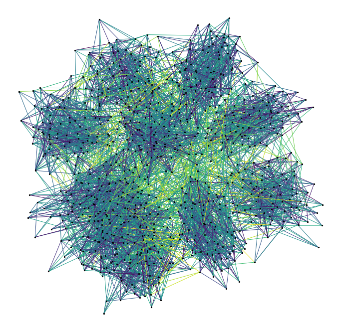
Our graph is a partition graph (10 partitions) with 800 edges, where edges inside the partitions have lower weight than edges between partitions. The colour highlighting shows the edge-weights: darker is smaller. You can just about make out the 10 partitions as darker clouds amongst the lighter edges.
Now let’s look at our distance.
def sp_dist(i,j):
    return nkx.dijkstra_path_length(G,i,j,weight='w')

randX = lambda : X[np.random.randint(nx)]
%timeit sp_dist(randX(),randX())
2.63 ms ± 254 µs per loop (mean ± std. dev. of 7 runs, 100 loops each)
That’s quite slow - around 250 times as slow as the Euclidean distance we calculated earlier! Now let’s compare our options: brute-force and ANNchor.
Brute Force
Given that we can’t use PyNNDescent or nmslib, we may well use brute-force simply because there’s not another option available to us.
from annchor import BruteForce
from annchor import compare_neighbor_graphs

start_time = time.time()

bruteforce = BruteForce(X,sp_dist)
bruteforce.get_neighbor_graph()

print('Brute Force Time: %5.3f seconds' % (time.time()-start_time))

error = compare_neighbor_graphs(neighbor_graph,
                                bruteforce.neighbor_graph,
                                k)

print('Brute Force Accuracy: %d incorrect NN pairs (%5.3f%%)' % (error,100*error/(k*nx)))
Brute Force Time: 304.143 seconds
Brute Force Accuracy: 0 incorrect NN pairs (0.000%)
That’s about 5 minutes. Remember, we only have 800 points in our data set! Imagine how badly this approach will scale.
ANNchor
ANNchor should take this problem in its stride. Let’s see how it compares.
from annchor import Annchor

k=15

start_time = time.time()

# Call ANNchor
ann = Annchor(X,
              sp_dist,
              n_anchors=20,
              n_neighbors=k,
              random_seed=5,
              n_samples=5000,
              p_work=0.15)

ann.fit()
print('ANNchor Time: %5.3f seconds' % (time.time()-start_time))


# Test accuracy
error = compare_neighbor_graphs(neighbor_graph,
                                ann.neighbor_graph,
                                k)
print('ANNchor Accuracy: %d incorrect NN pairs (%5.3f%%)' % (error,100*error/(k*nx)))
ANNchor Time: 38.200 seconds
ANNchor Accuracy: 2 incorrect NN pairs (0.017%)
That’s an order of magnitude faster than brute-force.